Forensic science lies at the intersections of legal, law enforcement, and scientific communities, each of which offer distinct approaches and perspectives to solving criminal justice concerns.

When it comes to specialized, scientific, or otherwise expert evidence, nearly all jurisdictions have two broad requirements for admissibility.

The first is relevance. Most attorneys are familiar that expert evidence must show some legally important fact to be made more or less probable by the presence of that evidence.

The second requirement legal authorities label “reliability,” which requires judges to keep junk science (or otherwise untrustworthy expert evidence) from reaching the fact-finder. Testimony such as, “the defendant’s DNA was found on his own gun,” may be irrelevant because whether or not the defendant touched a lawfully owned gun at some point, it has little concerning whether or not a crime was committed. Similarly, testimony around bitemark left on a victim from the defendant’s teeth may be unreliable if the method for determining such a conclusion is invalidated and unacceptable.

In any given case, the reliability varies depending upon the technique, the examiner, and the evidence itself; a “match” might be highly relevant or not relevant at all depending upon the circumstances of the case. A DNA match may establish that an individual’s DNA was found on an object, but it cannot establish how that DNA came to be there. Regardless of how strong the forensic evidence may be in the case, the investigator must still reach a conclusion about the plausibility of the narratives presented.

Two cases have created theoretically distinct standards for the admissibility of scientific or specialized evidence. Daubert, the federal standard created in 1993, requires the court to explore and measure the reliability of a technique, methodology, or theory itself. Daubert courts engage in a multi-factor balancing test weighing the falsifiability (or testability) of a theory; the known or potential rate of error; the presence of peer-reviewed articles; the general acceptance of the theory; and the presence of standards, among other potential factors.

By contrast Frye, founded in 1923, uses the acceptance of the relevant scientific community as a proxy for the reliability of the technique. Both standards are highly malleable. The best available research indicates no significant difference between states that employ a Frye standard over those that employ Daubert; however, the Daubert decision seems to have raised awareness about the possibility of junk science entering the courtroom and ignited challenges to scientific evidence of all sorts.

Reliability has a narrower meaning in a scientific context. When a scientist refers to reliability, they are referring to the consistency of the result. Low variation over time means high reliability. For a technique to be reliable in the legal sense, however, requires more than consistency; it also requires validity.

Validity asks whether the test or procedure measures what it is intended to measure. For example, many formerly accepted theories about fire investigation have undergone scientific scrutiny. Many investigators previously believed crazed glass was the result of extreme, rapid heating; yet, investigators were consistently wrong in their conclusions since crazed glass occurs when glass cools as well as when it heats up. Once controlled burn experiments and large-sample studies of fire debris were undertaken, recommendations against assigning probative value to crazed glass were reported.

A simpler analogy to accuracy and precision: when you throw darts at a dartboard, you may be very consistent or precise as all of the darts tightly cluster in one area. To be a successful dart player, you want something more than precision. If that cluster of darts is not on the bull’s-eye, then you haven’t been very accurate.

You need both precision and accuracy. Good scientific techniques need both reliability and validity.


http://forensictalks.blogspot.com/2011/02/accuracy-and-precision.html

Forensic scientists make claims about the world using certain methodologies or techniques. Unlike other scientists, forensic scientists cannot or do not know the likelihood that such a claim is correct. The pattern-matching disciplines (fingerprint examination, firearms comparison, handwriting comparison, etc.) are particularly plagued by such gaps in knowledge because of the subjective natures of the examinations.

Only recently have many forensic scientists begun to accept the probabilistic nature inherent in forensic conclusions. Traditionally, pattern-matching disciplines declare that two items come from the same source (inclusion), two items come from different sources (exclusion), or there’s not enough information to draw a conclusion either way (inconclusive). Examiners may strive to be conservative in their conclusions, but this categorization overstates the value of inclusions in and potentially understates the value of exclusions in all cases. Even when descriptions of likelihood are used – as in forensic document examination, which uses terms like “probability,” “strong probability,” and “very strong probability” – the basis of such descriptions are not scientifically grounded. Courts in many jurisdictions have ruled that a DNA match cannot be declared without statistics describing the probative value of the match because declaring a match in the absence of such statistics is meaningless. Courts generally do not treat the less scientifically grounded disciplines with the same rigor, however.

Even the most powerful of forensic tests have limitations, operate upon certain foundational assumptions, and require careful, meticulous interpretation. The National Academy of Sciences’ report,Strengthening Forensic Science: A Path Forward (NAS report), urges the forensic science community to adopt a research culture. 


From: Ulery BT, Hicklin RA, Buscaglia J, Roberts MA. Accuracy and reliability of forensic latent fingerprint decisions. Proc Natl Acad Sci USA. 2011 May 10;108(19):7733-8. Epub 2011 Apr 25.

In 2009, the National Academy of Sciences (NAS), following a mandate from Congress, released a report on the state of forensic science called Strengthening Forensic Science: A Path Forward. The National Research Council (NRC), an arm of the NAS, formed several committees to address the issue. They concluded that, among other things:

“[N]o forensic method other than nuclear DNA analysis has been rigorously shown to have the capacity to consistently and with a high degree of certainty support conclusions about ‘individualization’ (more commonly known as ‘matching’ of an unknown item of evidence to a specific known source). In terms of scientific basis, the analytically based disciplines generally hold a notable edge over disciplines based on expert interpretation. But there also are important variations among the disciplines relying on expert interpretation. For example, there are more established protocols and available research for the analysis of fingerprints than for bite marks. In addition, there also are significant variations within each discipline. Thus, not all fingerprint evidence is equally good, because the true value of the evidence is determined by the quality of the latent fingerprint image. In short, the interpretation of forensic evidence is not infallible. Quite the contrary. This reality is not always fully appreciated or accepted by many forensic science practitioners, judges, jurors, policymakers, or lawyers and their clients.”

Strengthening Forensic Science remains to date the most definitive and comprehensive declaration of the scientific community on the state of forensic science. The report has been used to challenge the admissibility and value of forensic evidence, the practices employed to develop forensic evidence, and the certainty with which a forensic expert can make conclusions. It has also spurred renewed interest in establishing the scientific foundations of many forensic sciences, such as fingerprint analysis and firearms comparison.

Some forensic sciences, such as DNA analysis or toxicological identification of common drugs, have been developed and utilized by the scientific community under rigorous, standardized procedures for reliable results with quantifiable degrees of error. For example, scientists run known samples of DNA or cocaine on their instruments over and over again to have a quantitative measure of how much the results can naturally vary and what the causes could be.

Many other forensic sciences were developed by law enforcement communities, and may lack standardized procedures and quantifiable degrees of error, and have only recently been the subject of scientific scrutiny. This has left courts and commentators in the awkward position of deciding how to handle testimony by individuals making claims about the world that sound scientific and have extensive precedent of being admissible, but currently lack a scientific foundation.

For example, one court dealt with forensic document examination testimony by instructing the jury in the following way:

You are about to hear the testimony of a forensic document examiner, who claims special qualification in the field of handwriting comparison, including the detection of forgeries. The Court has studied the nature of the skill claimed by forensic document examiners, and finds it to be closer to a practical skill, such as piloting a vessel, than to a scientific skill, such as that which might be developed by a chemist or a physicist. That is, although forensic document examiners may work in “laboratories,” and may rely on textbooks with titles like “The Scientific Examination of Documents,” forensic document examiners are not scientists – they are more like artisans, that is, skilled craftsmen.

The determination that a forensic document examiner is not a scientist does not suggest that this testimony is somehow inadequate, but it does suggest that his or her opinion may be less precise, less demonstrably accurate, than, say, the opinion of a chemist who testifies as to the results of a standard blood test.

In sum, the Court is convinced that forensic document examiners may be of assistance to you. However, their skill is practical in nature, and despite anything you may hear or have heard, it does not have the demonstrable certainty that some sciences have.

You may accept a forensic document examiner's testimony in whole, or you may reject it in whole. If you find that the field of forensic document examination is not sufficiently reliable, or that the particular document examiner is not sufficiently reliable, you are free to reject the testimony in whole. You may also accept the testimony in part, finding, as one possible example, that while the forensic document examiner has found significant similarities and differences between various handwriting samples, his or her conclusion as to the genuineness of a particular writing is in error, or is inconclusive. In any event, you should not substitute the forensic document examiner's opinion for your own reason, judgment, or common sense. I am not in any way suggesting what you should do. The determination of the facts in this case rests solely with you.

United States v. Starzecpyzel, 880 F. Supp. 1027, 1050-51 (S.D.N.Y. 1995)

Some courts see fit to exclude such testimony altogether, while other courts place limits on the certainty where forensic scientists can make their opinions.  Limiting language such as “is consistent with” or “cannot be excluded,” have been ascribed to pattern-matching examiners in some cases. Other courts have limited examiner testimony to pointing out the similar details or minutiae of a pattern used to draw conclusions.


From: http://www.fbi.gov/about-us/lab/forensic-science-communications/fsc/april2001/held.htm

The surfeit of crime over the past several years focused on forensic science has led to fears that jurors now have over-inflated expectations on the presentation of forensic evidence.

Jurors might expect that DNA or fingerprints can be easily developed in every case, and thereby create an impossibly high burden for the government to fulfill. Evidence of such effects are equivocal,[1] but since it is concerning to some, forensic scientists are now frequently put on the stand to explain the absence of such evidence.

Another concern is that jurors, when confronted with valuable forensic evidence, misconstrue evidence and its analysis as infallible. Having viewed all manner of cutting edge technology help to solve television crimes, there is a great deal of faith sometimes placed in any results labeled “forensic science,” whether or not it is merited. Forensic scientists as of late testify that the technique they used was infallible, 100% certain, or there was no chance of error. Such claims were never scientifically grounded and are now untenable.

Fingerprint examination has a long history of assisting criminal investigations. Over the past fifteen years, the discipline has faced increased scrutiny. The practice first came into wide use in the late 1800s and early 1900s as a means of verifying identities, later adopted to better assist criminal investigations.

In the controlled setting of a police department, fingerprints can either be electronically scanned or slowly rolled in ink, delivering varying qualities and movement. Any movement of the finger can lead to substantial distortions, while recovered fingerprints may not yet visible without some form of enhancement. Prints can be so distorted that it is impossible to match them to a known print. In other words, though there is a print, it is of "no value." This is a decision ultimately made by the fingerprint examiner.


Fingerprints vary in quality. From The Fingerprint Sourcebook.

Before being examined, prints must be located, developed, and enhanced. This procedure is handled by specialized police officers trained in the collection of physical evidence from crime scenes. Once properly photographed, stored and preserved, fingerprint examiners compare enhanced latent prints—along with known prints taken from the suspect, victim, or witness—is presented to the fact-finder.

Examiners distinguish the two types of differences with the prints they compare: discrepancies and distortions. A discrepancy is “a difference in two friction ridge impressions due to different sources of the impressions.” A distortion, by contrast, represents an “explainable” difference due to the nature of the print deposition or development. Fingers, as pliable, three-dimensional objects, do not fully adhere to prints presented, leaving the final decision on the cause to the examiner.

Each surface presents different challenges to develop fingerprints. Consider the number of surfaces our fingers come into contact with daily: metal doorknobs, plastic phone cases, disposable coffee cups, and more. Latent fingerprints are typically deposited in the sweat from our skin surface and are composed of roughly 98% water. With process, like each surface, possesses a myriad of challenges.

An extraordinarily wide range of fingerprint development methods exists: the commonality of crime scene officers dusting for prints is a single technique amidst series of physical and chemical steps. If they can be located and treated properly, fingerprints can be made to fluoresce with special lighting equipment and subsequently photographed.

If you look closely at your fingertips, you can see the ridges that make up a fingerprint. These ridges have overall flow patterns, usually categorized into arches, loops, and whorls.

Flow patterns are used to classify a fingerprint: to compare two prints, examiners must look at the minutiae (tiny characteristics of ridges). A ridge can end, or divide into more ridges. The patterns can puzzle examiners with more creases and scars.

Flow patterns – arch, loop, and whorl, respectively.

Before comparing a latent print to a known, examiners must determine whether a print has sufficient information for a comparison. Conventional standards have the examiner making a subjective, threshold decision about the value of the print: either it is “of value” or it has “no value.”

Most fingerprint examiners in the United States follow what is known as the ACE-V method. ACE-V stands for analysis, comparison, evaluation, and verification. The examiner analyzes the print in question, compares it to the known print, determines whether the prints are the same, and finally finds another examiner to verify the conclusions of the first. By convention, the examiner has three conclusions that she can reach: the fingerprints match (“identification” or “individualization”); the fingerprints don’t match (“exclusion”); or the examiner can’t reach a conclusion whether they match or not (an inconclusive result). Unfortunately, the broadness of the guidelines outlined by ACE-V has led to a wide diversity of comparison practices in the United States.

Fingerprint examination is not infallible. Highly qualified examiners have come to erroneous conclusions; examiners, when faced with new contexts for prints they have examined previously have altered their conclusions; and individuals have been wrongly convicted on the basis of fingerprint evidence. That is why highly detailed documentation is so critical to evaluate fingerprint evidence.

A recent report released by the National Institute of Standards and Technology on latent print examination, highlighted some of the strengths and weakness of the discipline, identified the sources of potential human error and made strong recommendations for thorough documentation of the basis for any conclusion reached by an examiner and inclusion in the report of any statements of important limitations to the conclusion reached.

As a bullet is fired from a gun, the barrel marks the softer metal of the bullet and its casing, leaving imprints. If police recover a gun (from a search, for example) and a bullet or cartridge casing (from the crime scene), then firearms analysts can compare the bullet and casing used in the crime with those test-fired from the gun, evaluating if the marks created will match.

Toolmark examiners generally place these marks into three categories—

Class characteristics: marks all weapons manufactured by the same company leave on the bullet or casing

Sub -class characteristics: microscopic marks that are due to idiosyncrasies in the manufacturing process

Individual characteristics: marks that only a specific weapon could make, often as a result of the "wear and tear" particular to that weapon

Beyond the difficulty in distinguishing between sub-class and individual characteristics, intra-gun variability can confound toolmark analysis, i.e. two bullets fired out of the same firearm will not share all of their characteristics with each other. Compounding this difficulty is the show-up nature of the examination. Test-fires and comparison of bullets/casing from the same make and model of gun are rarely performed in casework.

Business and manufacturing processes also have had an effect on firearms comparison. Both the consolidation of manufacturing companies and the streamlining of manufacturing processes have made guns considerably more uniform than they used to be, making the examination process more difficult.

With increasing uniformity in manufacture, there are simply fewer variations between any two guns that were made the same way.

Whether a firearms examiner can definitively individualize a bullet to a specific gun is under considerable debate, especially since there is an incredibly limited pool of data compiled to answer questions about how common/rare any particular trait is and how many discrepancies exist between cartridges fired from the same gun versus a different gun of the same model. A firearms examiner is asked to conclude whether the discrepancies they see are the result of the same or different weapon sans rubric, and their conclusion is their opinion about whether this similarity exceeds the “best agreement demonstrated” between marks left by known different weapons and “is consistent with agreement demonst

Reentry and Collateral Consequences

rated” by marks made by the same weapon (AFTE Theory of Identification.)

Still, a firearms examination can exclude a bullet as not having come from the gun in question, which can be critical in narrowing down leads, and can conclude that a bullet came from a limited class of weapons, which is valuable probative evidence in its own right.


Did these bullets come from the same gun or from different guns? Left: different; Right: same.

DNA analysis is considered the gold standard of forensic sciences because the scientific basis for profile comparison is well grounded, the error rates are quantifiable and usually very small, and the development procedure is highly reliable.

More goes into DNA analysis than the outsider might think. Forensic DNA analysts do not develop a full genomic profile (which would take a substantial amount of time and resources); rather, they look at very small parts of the genome where there is high variability among the population.

There are several forms of DNA analysis, but the most common one, STR, or short tandem repeat, examines the repetitions of base sequences at several locations of non-coding, nuclear DNA. Non-coding refers to the fact that there are locations on the DNA which do not code for specific protein sequences or functions, popularly referred to as “junk DNA”. We inherit one set of chromosomes from each parent and so have two alleles at each location (or locus).

What does a DNA report look like?

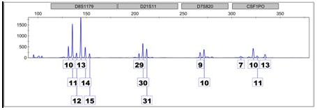
This is an electropherogram of four loci, represented by the grey boxes at the top, give the scientific nomenclature associated with that location on the genome.

The peaks signify alleles, or versions of that location, which are present in the sample. The number represents how many times a short sequence of nucleotide is repeated at a particular location on the genome in each version. The individual who contributed to this sample, for example, is a(12, 15) at D8, a (28, 29) at D2, a (8, 12) at D7, and a (9, 11) at CSF. This electropherogram is an example of a clean, single-source profile.

At D8, one parent contributed a chromosome with short sequence repeated 12 times, while the other parent contributed a chromosome where the same short sequence repeated 15 times. If an individual inherits the same allele from each parent, they are homozygous at that locus.

If the profile that the lab develops from evidence at the scene matches the profile of the defendant, a DNA expert will likely come to court to explain the analysis process and declare what the strength of the DNA evidence is. Usually, a statistic known as the random match probability describes the strength of the match between the two profiles.

The random match probability (RMP) reflects the profile’s rarity and gives us the likelihood that a randomly chosen, unrelated individual from a given population would have the same DNA profile observed in a sample. It relies on several key assumptions and, in some cases, can be controversial. In cases where the suspect has come under suspicion because of non-DNA evidence, and the DNA profile developed from the crime scene is a single-source full profile, most statisticians agree that the RMP is the most accurate measure of a coincidental match.

DNA, like other trace evidence, is only sometimes discovered and can be mixed, degraded, or contaminated. Even when DNA has been collected and properly stored and analyzed, the end result may only be a partial profile. Partial profiles don’t show alleles at all thirteen locations, but may only show alleles at varied locations, making the statistic associated less meaningful.

If there is a very small amount of DNA, interpretation of the results becomes considerably more complicated. Throughout analysis, the interpretation of artifacts like blobs, stutters, and off-ladder peaks can mean the difference between a match and an inconclusive result, or an inconclusive result and an exclusion. This is why labs are required to validate each piece of equipment and assess what levels of DNA input can still yield reliable results and are too low to be analyzed “below threshold”.

DNA Mixtures

When more than one individual has contributed DNA to a sample, the result is a mixture. The electropherogram above is an example because there are more than two peaks at multiple locations. Looking at D8 – the first locus on the left – we see six peaks of varying heights, indicating at least, or perhaps more than, three different contributors. Differences in peak height can be attributed to homozygous contributors or processes during the amplification phases of analysis.

How is a random match probability calculated?

If the sample comes from a single-source profile, calculating the random match probability is straightforward. The RMP relies on what is called the product rule: the probability of multiple independent events occurring is the product of the probabilities of each event occurring.

For example, the probability of getting two heads in a row on the flip of a fair coin is 0.5 * 0.5 or 0.25. There is a 50% chance that we get heads on the first flip and a 50% chance that we get heads on the second, thus a 25% chance that we would get two heads in a row.

In DNA analysis, each locus present qualifies as an independent event since the loci chosen have satisfied certain tests indicating that which alleles inherited at one location does not impact alleles inherited at another location. The frequency of each allele in the population can be used to calculate the frequency of the genotype at each locus, all of which can then be multiplied together. When some of the alleles are not present or if there are multiple contributors to the sample, calculating a statistic like the RMP becomes considerably challenging.

One of the costs of performing DNA analysis is the consumption of the biological material tested. In cases where only a small amount of DNA was collected, consuming all of the DNA evidence means that it can’t be retested. If a mistake occurs during testing (contamination, artifacts, etc.), it can only be reinterpreted. Forensic laboratories should consume no more than is necessary to test in order to preserve the possibility of a retest, as retests have prevented many miscarriages of justice.

A great deal of information about forensic STR typing can be found here.

Documentation and Review

Meticulous documentation bridges the gap between the raw evidence and the expert’s interpretation of that evidence. Without this, judges and juries are left with a bare opinion and are unable to judge the reasonableness of the inferences made by experts.

Consider that fingerprints, once developed, can be photographed, copied, and blown up. A fingerprint examiner should be able to identify the minutiae that identify or exclude a suspect through notes, diagrams, and photographs. By the same token, a firearms examiner can photograph and diagram his comparisons, and identify the striations that match between two bullets and explain apparent inconsistencies.

All members of the criminal justice system should embrace accurate, detailed documentation. It strengthens the value of the evidence presented, reduces errors by allowing internal and external review, and makes the presentation of evidence to a fact-finder easier and more convincing.

Scientific Training

Forensic science is the application of scientific theories, principles, and methods to issues of public facts. It may involve scientifically validated techniques, or a hypothesis about the aftermath of an accidental fire to be tested through the recreation of the scene and the fire. Either way, research is involved and reliability is accounted for through methodologically sound research experiments.  

Regardless of what forensic scientists are called upon to do, they must have a scientific background to do their jobs well well. Arson investigators must have an undergraduate background in physics and chemistry with hands-on training; fingerprint examiners study biology and statistics. The forensic science community, particularly in the wake of the NAS report, is going through a transitional period where the scientific and statistical foundations of many disciplines are being reevaluated.

As the forensic science community grows and coheres, current and incoming practitioners must have ways of getting the scientific training they need to properly evaluate their practices, in addition to the mentorship programs that are currently in place.

Contextual Bias

The NAS report acknowledges a concern regarding the effect of unintentional or subconscious cognitive bias in forensic practice. This phenomenon, often called “contextual bias,” be further studied[3], where influence of environment, extraneous detail, or “domain-irrelevant” information on decisions and judgments, can occur at each step of the analytical process that is open to any degree of subjectivity.

This issue is of particular concern in the “pattern-matching” disciplines (i.e. such as fingerprint and firearm/tool-mark examination) where the ultimate conclusion is inherently an analyst-subjective judgment based on the examiner’s training and experience.[4] A recent study brings attention the potential influence of this type of bias in the more scientifically-grounded fields of forensic science, such as DNA analysis, where the situation is one of a complicated mixture of profiles requiring subjective assessment to include or exclude a potential contributor.[5]

Some case-specific information may be relevant to the scientific analysis; however, routinely informing the individuals charged with obtaining scientific results of the age of the victim and brutality of the crime can create a one-sided lens through which the analysts view the evidence. This hints to incorrect assumptions, a see-what-you-expect-to-see confirmation bias, and unfounded conclusions.

“Context” may consist of a pro-prosecution culture in the lab, a conviction-based incentive structure, knowledge of additional investigative information, appreciation of law enforcement expectations or simple awareness of previous analyst conclusions. Whatever form it takes, extraneous input can significantly influence forensic results. Safeguarding against this type of subconscious bias requires heightening awareness of its empirically demonstrated existence, laboratory autonomy from law enforcement, or at the very least employing some type of “blinding” of analysts to this “domain-irrelevant” information.[6]

Forensic Science in General

Organizations

American Academy of Forensic Sciences

The American Society of Crime Laboratory Directors Laboratory Accreditation Board

The International Association of Identification (IAI)

The Consortium of Forensic Science Organizations

Publications

Strengthening Forensic Science in the United States: A Path Forward (National Academy of Sciences, 2009)

Modern Scientific Evidence: The Law and Science of Expert Testimony (Volume 4; Forensics), Faigman et al., (the latest edition is 2010-11)

The Need for a Research Culture in the Forensic Sciences (UCLA Law Review, 2011)

Forensic Science in the Media

Frontline: The Real CSI.

http://www.pbs.org/wgbh/pages/frontline/real-csi/

http://www.pbs.org/wgbh/pages/frontline/criminal-justice/real-csi/forensic-tools-whats-reliable-and-whats-not-so-scientific/

Post-mortem: Death Investigation in America (Propublica).

http://www.propublica.org/series/post-mortem

Shaken Baby Syndrome Faces New Questions in Court (NYTimes).

http://www.nytimes.com/2011/02/06/magazine/06baby-t.html

Trial by Fire: Did Texas Execute an Innocent Man?

http://www.newyorker.com/reporting/2009/09/07/090907fa_fact_grann

Convicted defendants left uninformed of forensic flaws found by Justice Dept.

http://www.washingtonpost.com/local/crime/convicted-defendants-left-uninformed-of-forensic-flaws-found-by-justice-dept/2012/04/16/gIQAWTcgMT_story.html

All About Forensic Science.

http://www.all-about-forensic-science.com/

When Memory Commits an Injustice.

http://online.wsj.com/article/SB10001424052702303815404577334040572533780.html

The Criminal Law Show: Forensic Evidence, http://www.wgxc.org/archives/4181

Science in court: Arrested development.

http://www.nature.com/news/science-in-court-arrested-development-1.10456

The CSI Effect

Donald Shelton et al., A Study of Juror Expectations and Demands Concerning Scientific Evidence: Does the CSI Effect Exist? Vanderbilt Journal of Entertainment & Technology Law, Vol. 9, p. 330, 2006.

http://ssrn.com/abstract=958224

N.J. Schweitzer and Michael Saks, The CSI Effect: Popular Fiction About

Forensic Science Affects Public Expectations About Real Forensic Science, Jurimetrics, Vol. 47, p. 357, Spring 2007.

http://ssrn.com/abstract=967706

Simon Cole and Rachel Dioso-Villa, CSI and its Effects: Media, Juries, and the Burden of Proof, New England Law Review, Vol 41, No. 3, 2007.

http://ssrn.com/abstract=1023258

Young Kim et al., Examining the ‘CSI-Effect’ in the Cases of Circumstantial Evidence and Eyewitness Testimony: Multivariate and Path Analyses, Journal of Criminal Justice, Vol. 37, No. 5, pp. 452-460, 2009

http://ssrn.com/abstract=1524228

Firearms

The Association of Firearm and Toolmark Examiners (AFTE).

http://www.afte.org/

The National Institute of Justice, Firearm Examiner Training Modules

http://www.nist.gov

Firearms ID.com: http://www.firearmsid.com/

National Integrated Ballistic Information Network: http://www.NIBIN.gov

Bureau of Alcohol, Tobacco, Firearms and Explosives: http://www.ATF.gov

DNA

The DNA Initiative. http://www.dna.gov/

SWGDAM Interpretation Guidelines for Autosomal STR Typing by Forensic DNA Labs.

http://www.fbi.gov/about-us/lab/codis/swgdam-interpretation-guidelines

STR Training Materials. http://www.cstl.nist.gov/biotech/strbase/training.htm

The Evaluation of Forensic DNA Evidence (National Research Council, 1996).

http://www.nap.edu/catalog.php?record_id=5141

DNA Technology in Forensic Science (National Research Council, 1992).

http://www.nap.edu/openbook.php?isbn=0309045878

Fundamentals of Forensic DNA Typing (Butler).

http://books.google.com/books?id=-OZeEmqzE4oC&printsec=frontcover&source=gbs_ge_summary_r&cad=0#v=onepage&q&f=false

Labs and consultants – for case-specific inquiries, contact PDS.

Technical Associates, Inc. http://www.tailabs.com/

Forensic Bioinformatics. http://www.bioforensics.com/

Chromosomal Labs-Bode Technology. http://www.chromosomal-labs.com/

NMS Labs. http://www.nmslab.com/Forensic-Services-Landing/

Fingerprints

The Fingerprint Sourcebook. http://www.nij.gov/pubs-sum/225320.htm

The Scientific Working Group on Friction Ridge Analysis, Study and Technology (SWGFAST).

http://www.swgfast.org/

Simon Cole’s faculty page. http://socialecology.uci.edu/faculty/scole

Ed German’s Latent Print Examination: Fingerprints, Palmprints and Footprints.

http://onin.com/fp/

Michele Triplett’s Fingerprint Dictionary. http://www.nwlean.net/fprints/e.htm

The Fingerprint Inquiry Scotland.

http://www.thefingerprintinquiryscotland.org.uk/inquiry/3127.html

Fire Investigation

The National Fire Protection Association (NFPA). http://www.nfpa.org

The International Association of Arson Investigators (IAAI).

http://firearson.com/

Scientific Fire Analysis, LLC http://www.firescientist.com/

Inter-FIRE Online. http://www.interfire.org/

Defense-oriented

Innocence Project. http://www.innocenceproject.org/

North Carolina Office of Indigent Defense. http://www.ncids.com/forensic/index.shtml

United States v. Ye Gon, United States District Court for the District of Columbia, Amicus Brady Pleading
PDS Letter to Judge Tallman, Chair, Judicial Conference Advisory Committee, on amending Rule 16
PDS Brady Handbook

Simms v. District of Columbia, Motion for Preliminary Injunction
Declaration of Frederick Simms
Simms v. District of Columbia, Opinion Granting Motion for Preliminary Injunction
Declaration of Keith Chung
Declaration of Sharlene Powell
Declaration of Nelly Moreira

McRae v. Grondolsky--Petitioner’s Objections to Magistrate’s Report & Recommendation
McRae v. Grondolsky--Petitioner’s Supplemental Brief
McRae Order on Petition for Habeas Corpus

Mark A. Briscoe & Sheldon A. Cypress v. Virginia Amicus Merits Brief
Jesse Jay Montejo v. Louisiana Amicus Merits Brief
Jesse Jay Montejo v. Louisiana Amicus Supplemental Brief
Bullcoming v. New Mexico Amici Brief
Sandy Williams v. Illinois Amicus Merits Brief

USAO initial report March 12, 2010
PDS response and call for wider review of cases involving FBI hair analysis April 14, 2010
USAO second report October 13, 2010
USAO rejection of PDS call for wider review and defense of FBI hair analysis November 15, 2010
PDS critique of microscopic hair analysis and response to USAO rejection of wider review December 16, 2010
Letter from Chief Judge Satterfield January 11, 2011
USAO final report December 9, 2011

Motion to Vacate Convictions on the Grounds of Actual Innocence December 9, 2009
Gov’t Response to Motion to Vacate Convictions December 14, 2009
Gov’t Motion to Join Gates Motion to Vacate Convictions December 18, 2009
Gov’t Letter to the Court December 18, 2009
Order Vacating Convictions December 18, 2009
Certificate of Actual Innocence May 4, 2010

Motion for Post-Conviction DNA Testing Under the Innocence Protection Act
Motion to Vacate Convictions and Dismiss Indictment with Prejudice on the Grounds of Actual Innocence Under the Innocence Protection Act

Motion to Vacate Conviction on the Grounds of Actual Innocence January 18, 2012
Supplement to Motion to Vacate Conviction and Motion to Vacate Conviction for Brady Violations March 13 2012

Goings v. CSOSA--Complaint
Goings v. CSOSA--Plaintiff’s Motion for Preliminary Injunction
Goings v. CSOSA--Order on Motion for Preliminary Injunction
Wills v. US Parole Commission et al.--Complaint
Wills v. US Parole Commission et al.--Plaintiff’s Motion for Partial Summary Judgment
Wills v. US Parole Commission et al.--Plaintiff’s Opposition to Motion to Dismiss